eurolig provides a toolkit to easily retrieve and analyze basketball generated data for the Euroleague with R. The package is mainly designed to work with two types of data: play-by-play data and shot location data. Although Euroleague’s first season was in 2000, play-by-play and shot location data is only available since the 2007/2008 season. This post introduces the latest realease of the package (v0.4.0) and shows how it could be used to do some basic analyses.
Changes in the new version
If you already used or knew about eurolig from an earlier post, you will notice quite some changes and added functionality. The previous (and first) version (0.0.0.900) of eurolig was very raw and experimental. In the new version (0.4.0) I haved added much more functionality and provided basic documentation.
The most important changes are:
camelCase for function names (instead of snake_case).
Removed the
plot_heatmap()functionality that produced assist pattern heatmaps.Output play-by-play data frames contain different variables.
Although there are a lot of changes, I did not keep old functions in the release because I think not many people are using the package. Old code will probably not work with the new realease. Note however that adapting old code to the new version will most likely be straight forward.
Required packages
You will need to install the eurolig package from its GitHub repository:
# install.packages("devtools")
devtools::install_github("solmos/eurolig")
In addition to eurolig, the following packages are needed to reproduce this post:
library(eurolig)
library(dplyr)
library(ggplot2)
Getting data
Datasets
Several datasets are included in the package. You can see all the available datasets by calling:
data(package = "eurolig")Sample datasets of play-by-play and shot location data are stored in samplepbp and sampleshots, respectively.
A particularly useful dataset in the package is gameresults. It contains all game results in the Euroleague from the 2001/2002 season to the 2018/2019 season. As you will see in the next section, this dataset can be useful to find the games you want to get data from.
Finally, if we need to find the name or identifying code of teams, the teaminfo dataset can be helpful.
extract functions
Functions that retrieve data from Euroleague’s website API start with the verb extract. You will need to be online for these functions to work.
The main functions to get data are:
extractPbp()for play-by-play data.extractShots()for shot location data.
These functions can only retrieve data from a single game. That means that if you want to get data for several games you will need to iterate the function over the games of interest. Note, however, that Euroleague’s robot.txt asks for a 15 (!) seconds delay between requests. Take this into consideration when requesting data for a lot of games.
Games are uniquely identified by a combination of season and game code. In order to indicate the extract functions what game we want to get data from, we need to pass the corresponding game code and season as arguments.
Let’s find the highest scoring games from the 2018/2019 season in the gameresults dataset:
games <- gameresults %>%
  filter(season == 2018) %>%
  mutate(total_points = points_home + points_away) %>%
  arrange(desc(total_points))

head(games)
## # A tibble: 6 x 14
## season phase round_name team_home points_home team_away points_away
## <int> <chr> <chr> <chr> <int> <chr> <int>
## 1 2018 RS Round 21 Herbalif… 104 AX Arman… 106
## 2 2018 RS Round 16 AX Arman… 111 Buducnos… 94
## 3 2018 RS Round 1 Real Mad… 109 Darussaf… 93
## 4 2018 RS Round 4 Herbalif… 91 CSKA Mos… 106
## 5 2018 RS Round 8 CSKA Mos… 99 Zalgiris… 97
## 6 2018 RS Round 25 CSKA Mos… 101 AX Arman… 95
## # … with 7 more variables: game_code <int>, date <chr>, round_code <int>,
## # game_url <chr>, team_code_home <chr>, team_code_away <chr>,
## # total_points <int>We can see that last season’s highest scoring game was the Herbalife Gran Canaria vs. AX Armani Exchange Olimpia Milan with 210 total points scored between the two teams. The identifying game code and season for this game are
games$season[1]## [1] 2018games$game_code[1]## [1] 168We can get play-by-play and shot location data for this game by passing these values as arguments to extractShots() and extractPbp():
game_shots <- extractShots(game_code = 168, season = 2018)
game_pbp <- extractPbp(168, 2018)
If you want to find games for the current season (not included in the gameresults dataset), you have two options: either look up the game code in the game’s url or use extractResults().
Analyzing play-by-play data
Play-by-play data provides a lot of information that traditional boxscore statistics fail to communicate. In the following subsections I am going to show how we can find the following information from play-by-play data:
Plus-Minus for one or more players.
On/Off statistics for one or more players.
Assists patterns within a team
For these analyses I am going to use the sample dataset samplepbp which contains the play-by-play data for all four games of the 2018/2019 Euroleague Final Four:
data("samplepbp")
glimpse(samplepbp)
## Observations: 2,121
## Variables: 29
## $ season <int> 2018, 2018, 2018, 2018, 2018, 2018, 2018, 2018, 2…
## $ game_code <int> 257, 257, 257, 257, 257, 257, 257, 257, 257, 257,…
## $ play_number <int> 2, 3, 4, 5, 6, 7, 8, 9, 10, 11, 12, 14, 15, 16, 1…
## $ team_code <chr> NA, "ULK", "IST", "ULK", "IST", "IST", "ULK", "IS…
## $ player_name <chr> NA, "DUVERIOGLU, AHMET", "DUNSTON, BRYANT", "MUHA…
## $ play_type <chr> "BP", "TPOFF", "TPOFF", "2FGM", "2FGA", "RBLK", "…
## $ time_remaining <chr> "10:00", "09:59", "09:59", "09:42", "09:19", "09:…
## $ quarter <dbl> 1, 1, 1, 1, 1, 1, 1, 1, 1, 1, 1, 1, 1, 1, 1, 1, 1…
## $ points_home <dbl> 0, 0, 0, 2, 2, 2, 2, 2, 2, 2, 2, 5, 5, 5, 5, 5, 5…
## $ points_away <dbl> 0, 0, 0, 0, 0, 0, 0, 0, 2, 2, 2, 2, 2, 2, 2, 2, 2…
## $ play_info <chr> "Begin Period", "", "", "Two Pointer (1/1 - 2 pt…
## $ seconds <dbl> 0, 1, 1, 18, 41, 41, 44, 45, 47, 56, 56, 67, 68, …
## $ home_team <chr> "Fenerbahce Beko Istanbul", "Fenerbahce Beko Ista…
## $ away_team <chr> "Anadolu Efes Istanbul", "Anadolu Efes Istanbul",…
## $ home <lgl> NA, TRUE, FALSE, TRUE, FALSE, FALSE, TRUE, FALSE,…
## $ team_name <chr> NA, "Fenerbahce Beko Istanbul", "Anadolu Efes Ist…
## $ last_ft <lgl> FALSE, FALSE, FALSE, FALSE, FALSE, FALSE, FALSE, …
## $ and1 <lgl> FALSE, FALSE, FALSE, FALSE, FALSE, FALSE, FALSE, …
## $ home_player1 <chr> "GREEN, ERICK", "GREEN, ERICK", "GREEN, ERICK", "…
## $ home_player2 <chr> "MELLI, NICOLO", "MELLI, NICOLO", "MELLI, NICOLO"…
## $ home_player3 <chr> "GUDURIC, MARKO", "GUDURIC, MARKO", "GUDURIC, MAR…
## $ home_player4 <chr> "MUHAMMED, ALI", "MUHAMMED, ALI", "MUHAMMED, ALI"…
## $ home_player5 <chr> "DUVERIOGLU, AHMET", "DUVERIOGLU, AHMET", "DUVERI…
## $ away_player1 <chr> "LARKIN, SHANE", "LARKIN, SHANE", "LARKIN, SHANE"…
## $ away_player2 <chr> "MOERMAN, ADRIEN", "MOERMAN, ADRIEN", "MOERMAN, A…
## $ away_player3 <chr> "MICIC, VASILIJE", "MICIC, VASILIJE", "MICIC, VAS…
## $ away_player4 <chr> "DUNSTON, BRYANT", "DUNSTON, BRYANT", "DUNSTON, B…
## $ away_player5 <chr> "SIMON, KRUNOSLAV", "SIMON, KRUNOSLAV", "SIMON, K…
## $ lineups <chr> "GREEN, ERICK - MELLI, NICOLO - GUDURIC, MARKO - …Plus-Minus
Plus-minus (+/-) measures the difference in team points scored and team points allowed while a player or a set of players of the same team are on the court. getPlusMinus() parses a play-by-play data frame with one or more games and returns the indicated player/s plus-minus statistic in each game.
Although widely used nowadays, it is important to note that raw plus-minus is very unstable and totally context dependent. It is, however, the building block for other more advanced stats such as RAPM or RPM.
Let’s check what Sergio Rodriguez (aka El Chacho) plus-minus was in the two Final Four games that he played in the 2018/2019 season:
chacho_pm <- getPlusMinus(pbp = samplepbp, players = "RODRIGUEZ, SERGIO")
# Select only a few columns so that data frame fits in the document
chacho_pm %>%
  select(game_code, team_code_opp, poss, poss_opp, plus_minus)
## # A tibble: 2 x 5
## game_code team_code_opp poss poss_opp plus_minus
## <int> <chr> <dbl> <dbl> <dbl>
## 1 258 MAD 44 42 8
## 2 260 IST 24 25 -10Note that you can find the plus-minus statistic for combinations of players by entering a character vector with the player names in the players argument.
On/Off Statistics
On/Off statistics for a player or a set of players measure team statistics when the player or players where on the court and when they were on the bench.
You can use getOnOffStats() to find on/off statistics. For instance, I can find out how Real Madrid did when Rudy and Ayón were together on the court versus when both were on the bench in the two games played in the 2018/2019 Final Four.
getOnOffStats(pbp = samplepbp, players = c("FERNANDEZ, RUDY", "AYON, GUSTAVO"))## # A tibble: 8 x 28
## season game_code players on type team_code home fg2a fg2m fg2_pct
## <int> <int> <chr> <lgl> <chr> <chr> <lgl> <int> <int> <dbl>
## 1 2018 258 FERNAN… TRUE defe… CSK TRUE 5 1 0.2
## 2 2018 258 FERNAN… TRUE offe… MAD FALSE 3 2 0.667
## 3 2018 259 FERNAN… TRUE offe… MAD FALSE 20 14 0.7
## 4 2018 259 FERNAN… TRUE defe… ULK TRUE 15 7 0.467
## 5 2018 258 FERNAN… FALSE defe… CSK TRUE 33 16 0.485
## 6 2018 258 FERNAN… FALSE offe… MAD FALSE 43 22 0.512
## 7 2018 259 FERNAN… FALSE offe… MAD FALSE 15 9 0.6
## 8 2018 259 FERNAN… FALSE defe… ULK TRUE 17 9 0.529
## # … with 18 more variables: fg3a <int>, fg3m <int>, fg3_pct <dbl>,
## # fga <int>, fgm <int>, fg_pct <dbl>, fta <int>, ftm <int>,
## # ft_pct <dbl>, orb <int>, drb <int>, tov <int>, ast <int>, stl <int>,
## # cpf <int>, blk <int>, pts <dbl>, poss <dbl>Note that getOnOffStats() returns 4 rows per game corresponding to:
Team statistics when players were on the court together.
Opposing team statistics when players were on the court together.
Team statistics when players were on the bench together.
Opposing team statistics when players were on the bench together.
Assists patterns
Play-by-play data allows us to find out who assists who on assisted baskets. The function getAssists() returns a data frame with the passer and the shooter (plus more contextual information) for all assisted baskets in the input play-by-play data.
I am going to use getAssists() and some data wrangling to find out the most common assists in CSKA Moscow during the two games of the 2018/2019 Final Four:
assists_csk <- getAssists(pbp = samplepbp, team = "CSK")
assists_csk %>%
  count(passer, shooter) %>%
  arrange(desc(n))
## # A tibble: 25 x 3
## passer shooter n
## <chr> <chr> <int>
## 1 CLYBURN, WILL HIGGINS, CORY 2
## 2 DE COLO, NANDO HACKETT, DANIEL 2
## 3 HACKETT, DANIEL HUNTER, OTHELLO 2
## 4 RODRIGUEZ, SERGIO HINES, KYLE 2
## 5 CLYBURN, WILL DE COLO, NANDO 1
## 6 DE COLO, NANDO CLYBURN, WILL 1
## 7 DE COLO, NANDO HUNTER, OTHELLO 1
## 8 DE COLO, NANDO KURBANOV, NIKITA 1
## 9 DE COLO, NANDO PETERS, ALEC 1
## 10 HACKETT, DANIEL CLYBURN, WILL 1
## # … with 15 more rowsAnalyzing shot location data
Shot location data specifies the x and y coordinates of every jump shot taken during a game. This data can be useful for, say, identifying shooting location tenedencies on offense of a given player/team, showing what spots on the court a player is most effective at, or analyzing what type of shots a team allows its opponents.
For the following analysis, I am going to use the sampleshots dataset, which contains the shot location data for the four games in the 2018/2019 Final Four.
glimpse(sampleshots)## Observations: 490
## Variables: 25
## $ season <dbl> 2018, 2018, 2018, 2018, 2018, 2018, 2018, 2018, 20…
## $ game_code <int> 257, 257, 257, 257, 257, 257, 257, 257, 257, 257, …
## $ num_anot <int> 5, 6, 10, 14, 16, 18, 21, 25, 27, 30, 31, 33, 34, …
## $ team_code <chr> "ULK", "IST", "IST", "ULK", "IST", "ULK", "IST", "…
## $ player_id <chr> "P001324", "P003048", "P003048", "P005159", "P0018…
## $ player_name <chr> "MUHAMMED, ALI", "DUNSTON, BRYANT", "DUNSTON, BRYA…
## $ action_id <chr> "2FGM", "2FGA", "2FGM", "3FGM", "2FGA", "2FGA", "2…
## $ action <chr> "Two Pointer", "Missed Two Pointer", "Two Pointer"…
## $ points <int> 2, 0, 2, 3, 0, 0, 0, 3, 0, 3, 0, 3, 3, 2, 2, 2, 0,…
## $ coord_x <dbl> 1.1428571, -0.3163265, -0.1836735, -5.9489796, 1.9…
## $ coord_y <dbl> 2.279082, 2.717857, 2.207653, 6.177041, 2.462755, …
## $ zone <chr> "C", "B", "B", "H", "C", "C", "B", "H", "G", "I", …
## $ fastbreak <lgl> FALSE, FALSE, FALSE, FALSE, FALSE, FALSE, FALSE, T…
## $ second_chance <lgl> FALSE, FALSE, TRUE, FALSE, FALSE, FALSE, FALSE, FA…
## $ off_turnover <lgl> FALSE, FALSE, FALSE, FALSE, FALSE, FALSE, FALSE, T…
## $ minute <int> 1, 1, 1, 2, 2, 2, 3, 3, 3, 4, 4, 4, 4, 5, 5, 6, 6,…
## $ console <chr> "09:42", "09:19", "09:13", "08:53", "08:29", "08:0…
## $ points_a <int> 2, 2, 2, 5, 5, 5, 5, 5, 5, 5, 5, 5, 8, 8, 10, 12, …
## $ points_b <int> 0, 0, 2, 2, 2, 2, 2, 5, 5, 8, 8, 11, 11, 13, 15, 1…
## $ utc <chr> "20190517160232", "20190517160256", "2019051716030…
## $ make <lgl> TRUE, FALSE, TRUE, TRUE, FALSE, FALSE, FALSE, TRUE…
## $ quarter <int> 1, 1, 1, 1, 1, 1, 1, 1, 1, 1, 1, 1, 1, 1, 1, 1, 1,…
## $ seconds <dbl> 18, 41, 47, 67, 91, 117, 130, 146, 176, 185, 203, …
## $ team_code_a <chr> "ULK", "ULK", "ULK", "ULK", "ULK", "ULK", "ULK", "…
## $ team_code_b <chr> "IST", "IST", "IST", "IST", "IST", "IST", "IST", "…You can see in addition to the x-y coordinates, coord_x and coord_y, there are variables that give you more contextual information such as the player that took the shot, the time in the clock when the shot was taken or whether the shot was after an offensive rebound. These variables can help you filter specific shot types.
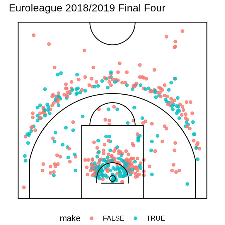
The function plotShotChart() allows you to show graphically where the shots were taken on the court and colored according to whether the shot went in (green) or not (red). The returned object is a ggplot object that we can customize with ggplot2 functions:
plotShotchart(sampleshots) +
  labs(title = "Euroleague 2018/2019 Final Four") +
  theme(legend.position = "bottom")